Plot Method for Kvalseth's R-squared Objects

Visualizes the different R-squared definitions or provides a diagnostic observed-vs-predicted plot to understand the model fit.

Usage

plot_kvr2(
  x,
  type = c("auto", "linear", "power"),
  plot_type = c("both", "r2", "diag"),
  ...
)

Arguments

x: An object of class lm.
type: Character string. Selects the model type: "linear", "power", or "auto" (default). In "auto", the function detects if the dependent variable is log-transformed.
plot_type: A string specifying the plot layout: "both" (default) displays the bar plot and diagnostic plot side-by-side, "r2" shows only the R-squared comparison, and "diag" shows only the observed-vs-predicted plot.
...: Currently ignored.

Value

The return value depends on the plot_type argument:

For "r2" and "diag": Returns a ggplot object that can be further customized.
For "both": Generates a combined plot using the grid system and returns the input object x invisibly.

Details

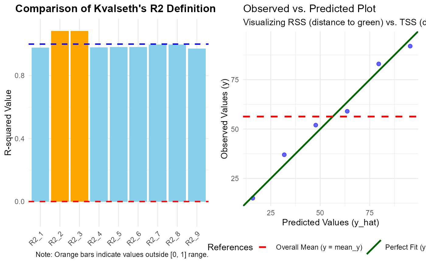
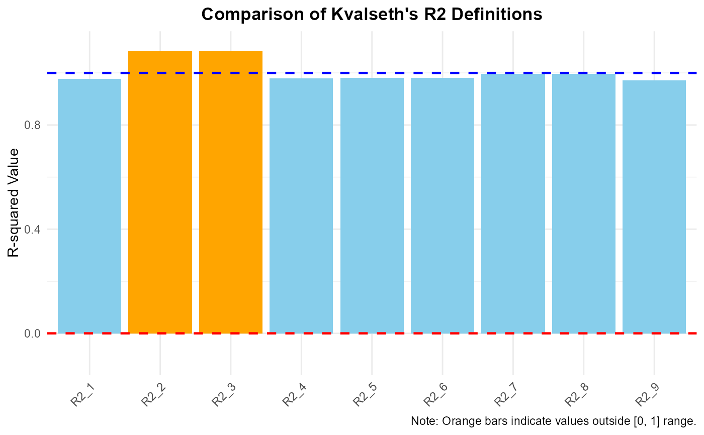
When plot_type = "r2", the function creates a bar plot comparing all nine definitions. Bars are colored based on their validity:

Skyblue: Standard values between 0 and 1.
Orange: Values exceeding 1.0 or falling below 0.0 (warnings).

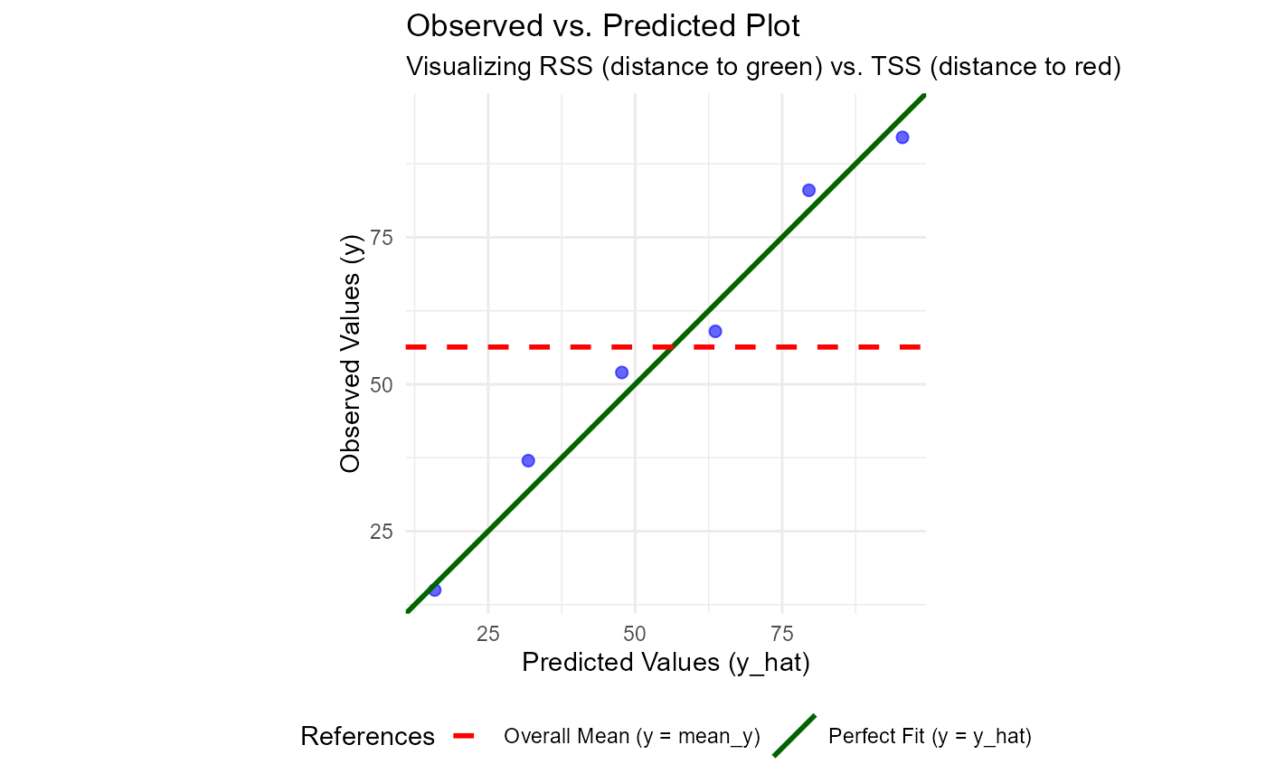
When plot_type = "diag", the function displays a scatter plot of observed vs. predicted values. Two reference lines are added:

Darkgreen Solid Line: The 1:1 "perfect fit" line (RSS reference).
Red Dashed Line: The overall mean of the observed data (TSS reference).

If the data points are closer to the red dashed line than the green solid line, \(R^2_1\) will be negative.

Combined View (plot_type = "both"): Automatically configures the plotting device to show both plots simultaneously for a comprehensive model evaluation.

Examples

df1 <- data.frame(x = 1:6, y = c(15, 37, 52, 59, 83, 92))
model <- lm(y ~ x - 1, data = df1) # No-intercept model
plot_kvr2(model)

# Compare all definitions
plot_kvr2(model, plot_type = "r2")


# Diagnostic plot to see why some R2 might be problematic
plot_kvr2(model, plot_type = "diag")