The kvr2 package provides functions to calculate nine types of coefficients of determination (\(R^2\)) as classified by Kvalseth (1985).
Overview
The coefficient of determination, \(R^2\), is one of the most common metrics for assessing model fit. However, its mathematical definition is not unique. While various formulas yield identical results in standard linear regression with an intercept, they can diverge significantly—sometimes producing negative values or values exceeding 1—when applied to:
- Models without an intercept (No-intercept models)
- Power regression models
- Other fits via transformations (e.g., log-log models)
Scope and Compatibility
This package is specifically designed for models that can be represented as lm objects in R. This includes:
- Standard Linear Models (with an intercept)
-
No-intercept Models (e.g.,
lm(y ~ x - 1)) -
Power Regression Models (fitted via log-transformation, such as
lm(log(y) ~ log(x)))
Note: This package does not support general non-linear least squares (nls) or other complex non-linear modeling frameworks. It focuses on the mathematical sensitivity of \(R^2\) within the context of linear estimation and its common transformations.
Educational Purpose: Demystifying
The primary goal of kvr2 is not to provide a definitive “best” for every scenario, but to serve as an educational and diagnostic resource. Many users rely on the single value provided by standard software, but as this package demonstrates, that value is sensitive to the underlying mathematical definition and the software’s internal defaults.
Through this package, users can:
- Understand Mathematical Sensitivity: Observe firsthand how different algebraic formulas (eight + one definitions) can lead to dramatically different interpretations of the same model fit, especially in non-intercept models.
- Diagnose Negative: It is imperative to acknowledge that a negative (typically in) should not be interpreted as a “bug”; rather, it functions as a critical diagnostic signal. This signal indicates that the model predicts outcomes that fall below the mean of a simple horizontal line.
- Evaluate Robustness and Transformations: Explore Kvalseth’s recommendations for using for consistency and for robustness against outliers, and see how behaves when models are fitted in transformed spaces (e.g., log power regression models).
Formulas Included
The package calculates nine indices based on Kvalseth (1985):
- \(R^2_1\) to \(R^2_8\): A classification of existing and historical formulas used in statistical literature and software.
- \(R^2_9\): A robust version of the coefficient of determination based on median absolute deviations, as proposed in the original paper.
Installation
You can install the released version of kvr2 from CRAN with:
install.packages("kvr2")You can install the development version of kvr2 like so:
remotes::install_github("indenkun/kvr2")Usage and Examples
kvr2 provides a simple way to observe how different \(R^2\) definitions behave across various model specifications.
1. Basic Usage: Consistency and Divergence
In standard linear models with an intercept, most \(R^2\) definitions yield identical results. However, they can diverge significantly in models without an intercept or in power regression models.
library(kvr2)

# Dataset from Kvalseth (1985)
df1 <- data.frame(x = 1:6, y = c(15, 37, 52, 59, 83, 92))

# Case A: Linear regression with intercept (Values are consistent)
model_int <- lm(y ~ x, data = df1)
r2(model_int)
#> R2_1 :  0.9808
#> R2_2 :  0.9808
#> R2_3 :  0.9808
#> R2_4 :  0.9808
#> R2_5 :  0.9808
#> R2_6 :  0.9808
#> R2_7 :  0.9966
#> R2_8 :  0.9966
#> R2_9 :  0.9778
#> ---------------------------------
#> (Type: linear, with intercept, n: 6, k: 2)

# Case B: Linear regression without intercept (Values diverge)
model_no_int <- lm(y ~ x - 1, data = df1)
results <- r2(model_no_int)
results
#> R2_1 :  0.9777
#> R2_2 :  1.0836
#> R2_3 :  1.0830
#> R2_4 :  0.9783
#> R2_5 :  0.9808
#> R2_6 :  0.9808
#> R2_7 :  0.9961
#> R2_8 :  0.9961
#> R2_9 :  0.9717
#> ---------------------------------
#> (Type: linear, without intercept, n: 6, k: 1)
Observation: In Case B, notice that \(R^2_2\) and \(R^2_3\) exceed 1.0. This demonstrates why choosing the correct definition is critical for models without an intercept.
2. Accessing Calculated Values
The r2() function returns a list object. While the output is formatted for readability, you can easily access individual values for further analysis or reporting.
# Accessing specific R2 values from the result object
results$r2_1
#>      r2_1
#> 0.9776853

results$r2_9
#>      r2_9
#> 0.9717156

# You can also use it in your custom functions or data frames
my_val <- results$r2_1
3. Visualizing the Sensitivity of R-squared
To better understand the divergence between these definitions, the kvr2 package provides a specialized plotting function. When you apply plot_kvr2() to your model, it displays both the comparison of \(R^2\) definitions and a diagnostic observed-vs-predicted plot.
# Example with the forced no-intercept model
plot_kvr2(model_no_int)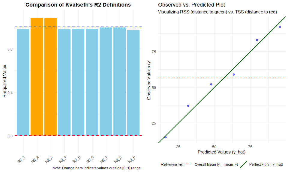
In the resulting side-by-side plot:
Left Panel: Shows which definitions are most affected by the intercept constraint.
Right Panel: Reveals if the model (green line) is performing worse than the simple average (red line).
4. Model Comparison with Error Metrics
To complement \(R^2\) analysis, use comp_fit() to evaluate models via standard error metrics such as RMSE, MAE, and MSE.
comp_fit(model_no_int)
#> RMSE :  3.9008
#> MAE :  3.6520
#> MSE :  18.2593
#> ---------------------------------
#> (Type: linear, without intercept, n: 6, k: 1)
For details, refer to the documentation for each function.
5. Direct Comparison of Constraints
The comp_model() function allows you to instantly see the impact of the intercept constraint. In the example below, notice how \(R^2_2\) remains misleadingly high in the no-intercept model, whereas \(R^2_1\) drops, reflecting the true decrease in predictive accuracy relative to the mean.
res_comp <- comp_model(model_no_int)
res_comp
#> model             |   R2_1 |   R2_2 |   R2_3 |   R2_4 |   R2_5 |   R2_6
#> -----------------------------------------------------------------------
#> with intercept    | 0.9808 | 0.9808 | 0.9808 | 0.9808 | 0.9808 | 0.9808
#> without intercept | 0.9777 | 1.0836 | 1.0830 | 0.9783 | 0.9808 | 0.9808
#>
#> model             |   R2_7 |   R2_8 |   R2_9 |   RMSE |    MAE |     MSE
#> ------------------------------------------------------------------------
#> with intercept    | 0.9966 | 0.9966 | 0.9778 | 3.6165 | 3.5238 | 19.6190
#> without intercept | 0.9961 | 0.9961 | 0.9717 | 3.9008 | 3.6520 | 18.2593
#> ---------------------------------
#>
#> Note: Some R2 values exceed 1.0 or are negative, indicating that these definitions may be inappropriate for the no-intercept model.
The power of kvr22 lies in its ability to visually demonstrate why certain \(R^2\) definitions fail when an intercept is removed. By calling plot() on a comp_model object, you generate a comprehensive 2x2 Diagnostic Dashboard.
# Generate the dashboard
plot(res_comp)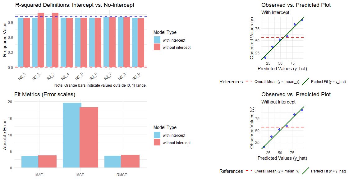
What the dashboard reveals:
- R-squared Comparison (Top-Left): Side-by-side bars for all 9 definitions. Orange bars instantly flag “illegal” values (e.g., \(R^2 > 1\) or \(R^2 < 0\)), which are common in no-intercept models.
- Fit Metrics (Bottom-Left): Direct comparison of RMSE, MAE, and MSE to see the actual error trade-off.
- Diagnostic Plots (Right Column): Observed vs. Predicted scatter plots.
- The Green line represents a perfect fit (\(y = \hat{y}\)).
- The Red dashed line represents the global mean (\(y = \bar{y}\)).
- If the data points are closer to the red line than the green line, \(R^2_1\) will be negative—a clear visual proof of model poorness.
Note: This dashboard is built using the
gridsystem. While it provides a complete overview, it cannot be modified withggplot2’s+operator. For customized single plots, useplot_kvr2(model, plot_type = "r2")orplot_diagnostic(model).
References
Kvalseth, T. O. (1985). Cautionary Note about \(R^2\). The American Statistician, 39(4), 279-285. DOI: 10.1080/00031305.1985.10479448